suppressPackageStartupMessages({
  library(dplyr)
  library(tidyr)
  library(lubridate)
  library(purrr)
  library(nasapower)
  library(ggplot2)
  library(forcats)
  library(jsonlite)
  library(tibble)
  library(readxl)
  library(lme4)
  library(sjPlot)
  library(metafor)
  library(patchwork)
})Data Analysis
Library import
Load the necessary packages.
Auxiliary variables definition
Key parameters definition. Thresholds used in the response curves and to identify analog years. Threshold values for temperature and relative humidity were selected to represent critical conditions associated with wheat blast development, including both winter conditions and the heading period. Sigmoidal response functions were parameterized using slope coefficients to control the sensitivity of the indices to deviations from these thresholds.
A set of sentinel sites was defined to represent key wheat-growing regions across southern Brazil, Uruguay, and Argentina, capturing a broad latitudinal and climatic gradient. For each location, geographic coordinates and a site-specific temporal window corresponding to the wheat heading period were specified. These periods are defined using fixed calendar dates and subsequently converted to day-of-year format to facilitate alignment with daily climate data.
# Threshold and Benchamark -----------------------------------------------------
CFG <- list(
  T0    = 15, # Winter temperature threshold
  RH0   = 90, # Relative Humidity threshold
  k_RH  = 2, # Response curve slope
  T_low = 16, # Heading period  low temperature threshold
  T_high= 26, # Heading period  high temperature threshold
  k_T   = 2, # Response curve slope
  benchmark_year = 2023, # Benchmark year
  eps            = 0.05,  # Quantile tolerance
  k_closest      = 10,    # Number of distance analog years
  benchmark_site = "Passo Fundo (BR)" # Benchmark site name
)

# CORDEX members dataframe list -----------------------------------------------
member_files <- list.files(
  "D:/Igor_Masters/paper2_analog_years/CordexInputData/rcp85",
  pattern = "^Member.*\\.xlsx$",
  full.names = TRUE
)

# Sentinel sites dataframe ----------------------------------------------------
sentinels <- tibble::tribble(
  ~country,   ~zone_gradient,                 ~site,                 ~lat,    ~lon,    ~start_month, ~start_day, ~end_month, ~end_day,
  "Brazil",   "Western RS (continental)",     "Santa Rosa (BR)",     -27.87,  -54.48,   8L,           15L,        9L,         15L,
  "Brazil",   "Central–North RS (reference)", "Passo Fundo (BR)",    -28.26,  -52.40,   9L,           15L,       10L,         15L,
  "Brazil",   "Eastern RS (highlands)",       "Vacaria (BR)",        -28.51,  -50.94,  10L,            1L,       10L,         31L,
  "Uruguay",  "Northern Litoral",             "Artigas-Salto (UY)",  -30.40,  -56.50,  10L,            1L,       10L,         31L,
  "Argentina","Zone II (North Pampas)",       "Pergamino (AR)",      -33.89,  -60.57,  10L,            1L,       10L,         31L,
  "Argentina","Zone IV (South Pampas)",       "Tandil (AR)",         -37.32,  -59.13,  11L,            1L,       11L,         30L
) %>%
  mutate(sentinel_id = row_number()) %>%
  select(sentinel_id, everything()) %>%
  mutate(
    start_doy = yday(make_date(2001, start_month, start_day)),
    end_doy   = yday(make_date(2001, end_month, end_day))
  )
sentinels
# A tibble: 6 × 12
sentinel_id country zone_gradient site lat lon start_month start_day
<int> <chr> <chr> <chr> <dbl> <dbl> <int> <int>
1 1 Brazil Western RS (con… Sant… -27.9 -54.5 8 15
2 2 Brazil Central–North R… Pass… -28.3 -52.4 9 15
3 3 Brazil Eastern RS (hig… Vaca… -28.5 -50.9 10 1
4 4 Uruguay Northern Litoral Arti… -30.4 -56.5 10 1
5 5 Argentina Zone II (North … Perg… -33.9 -60.6 10 1
6 6 Argentina Zone IV (South … Tand… -37.3 -59.1 11 1
# ℹ 4 more variables: end_month <int>, end_day <int>, start_doy <dbl>,
# end_doy <dbl>DT::datatable(
sentinels,
options = list(
pageLength = 10,
scrollX = TRUE
)
)Functions definition
Define functions to calculate the climatic indices and classify distance, quantile and conservative analogs. Auxiliary functions to create the sigmoid response curves for S_head, graphics plots and a function to input and prepare CORDEX members ensemble dataframe.
calc_ET_JJA (Winter (JJA) Thermal Favorability Index): Quantified using the accumulated temperature exceedance during June–August (JJA), calculated as the sum of daily temperatures above a defined threshold (15ºC). This metric captures the intensity of anomalously warm winter conditions. To facilitate interannual comparison, an empirical cumulative distribution function (ECDF) was applied to derive a standardized temperature index.
calc_S_head (Hygrothermal suitability index): Climatic suitability during the wheat heading period, represented by combining temperature and relative humidity responses. Suitability was modeled using sigmoid-based response functions, where relative humidity enhances suitability above a critical threshold, and temperature contributes within an optimal range defined by lower and upper bounds. Daily suitability values were averaged over a site-specific heading window to produce a seasonal index, which was subsequently standardized using the ECDF approach.
To quantify similarity with the benchmark year, a Euclidean distance metric is computed using standardized anomalies of both indices (calc_distance_to_benchmark). This approach ensures that differences in scale between variables do not bias the distance calculation.
Analog years were identified using two complementary criteria (identify_within_site_analogs). Quantile analogs are years with index values comparable to or exceeding those of the benchmark within a defined tolerance. Second, distance analogs area the 10 closest years in terms of multivariate climatic similarity. The intersection of these two methods defines a subset of years that simultaneously satisfy both criteria, this conservative classification that defines what will be considered the analog years.
# Winter (JJA) Thermal Favorability Index: ET_JJA and I_temp ----------------------
calc_ET_JJA <- function(df_daily, T0 = 15) {
  df_daily %>%
    filter(mon %in% c(6, 7, 8)) %>%  # JJA
    group_by(sentinel_id, country, site, lat, lon, year) %>%
    summarise(
      ET_JJA = sum(pmax(0, T2M - T0), na.rm = TRUE),
      n_days_JJA = dplyr::n(),
      .groups = "drop"
    ) %>%
    group_by(sentinel_id) %>%
    mutate(I_temp = ecdf(ET_JJA)(ET_JJA)) %>%
    ungroup()
}

# Hygrothermal suitability index: S_head and I_head -------------------------------
sigmoid <- function(x) 1 / (1 + exp(-x))

f_RH <- function(RH, RH0 = 90, k_RH = 2) {
  sigmoid((RH - RH0) / k_RH)
}

f_T <- function(T, T_low = 16, T_high = 26, k_T = 2) {
  sigmoid((T - T_low) / k_T) * sigmoid((T_high - T) / k_T)
}

calc_S_head <- function(df_daily, sentinels,
                        RH0 = 90, k_RH = 2,
                        T_low = 16, T_high = 26, k_T = 2) {

  df2 <- df_daily %>%
    left_join(
      sentinels %>% select(sentinel_id, start_doy, end_doy),
      by = "sentinel_id"
    ) %>%
    mutate(
      head_start_date = as.Date(start_doy - 1,
                                origin = paste0(year, "-01-01")),
      head_end_date   = as.Date(end_doy - 1,
                                origin = paste0(year, "-01-01")),

      in_head_window = if_else(
        start_doy <= end_doy,
        date >= head_start_date & date <= head_end_date,
        date >= head_start_date | date <= head_end_date  # future wrap safety
      ),
      S_d = f_RH(RH2M, RH0, k_RH) * f_T(T2M, T_low, T_high, k_T)
    )

  df2 %>%
    filter(in_head_window) %>%
    group_by(sentinel_id, country, site, lat, lon, year) %>%
    summarise(
      S_head = mean(S_d, na.rm = TRUE),
      n_days_head = dplyr::n(),
      .groups = "drop"
    ) %>%
    group_by(sentinel_id) %>%
    mutate(I_head = ecdf(S_head)(S_head)) %>%
    ungroup()
}

# Calculate Euclidean distance ----------------------------------------------------
calc_distance_to_benchmark <- function(df_site, bench_year) {
  b <- df_site %>% filter(year == bench_year)
  if (nrow(b) != 1) {
    df_site$D <- NA_real_
    return(df_site)
  }

  sd_ET <- sd(df_site$ET_JJA, na.rm = TRUE)
  sd_S  <- sd(df_site$S_head, na.rm = TRUE)

  if (!is.finite(sd_ET) || sd_ET == 0) sd_ET <- NA_real_
  if (!is.finite(sd_S)  || sd_S  == 0) sd_S  <- NA_real_

  df_site %>%
    mutate(
      D = sqrt(
        ((ET_JJA - b$ET_JJA) / sd_ET)^2 +
          ((S_head - b$S_head) / sd_S)^2
      )
    )
}

# Classify analogs ----------------------------------------------------------------
identify_within_site_analogs <- function(df_indices,
                                         benchmark_year = 2023,
                                         eps = 0.05,
                                         k_closest = 10) {
  df_indices %>%
    group_by(sentinel_id) %>%
    group_modify(~{
      df_site <- .x %>% arrange(year)

      bq <- df_site %>% filter(year == benchmark_year) %>%
        select(I_temp, I_head)

      if (nrow(bq) != 1) {
        df_site$analog_quantile <- FALSE
        df_site$analog_distance <- FALSE
        df_site$analog_both     <- FALSE
        df_site$D <- NA_real_
        return(df_site)
      }

      # A) quantile analog (kept as in your code: one-sided tolerance)
      df_site <- df_site %>%
        mutate(
          analog_quantile =
            (I_temp >= (bq$I_temp - eps)) &
            (I_head >= (bq$I_head - eps))
        )

      # B) distance analog (k closest)
      df_site <- calc_distance_to_benchmark(df_site, benchmark_year) %>%
        arrange(D) %>%
        mutate(analog_distance = row_number() <= k_closest) %>%
        arrange(year)

      # overlap
      df_site %>% mutate(analog_both = analog_quantile & analog_distance)
    }) %>%
    ungroup()
}

# CORDEX members dataframes input and Indices calculation -------------------------
run_member_indices <- function(member_path, Era5_daily, sentinels, CFG, CrossSiteFlag=FALSE) {
  MemberId <- tools::file_path_sans_ext(basename(member_path))
  df_daily <- read_excel(member_path) %>%
    filter(year >= 2024, year <= 2055) %>%
    distinct()
  df_daily$site <- gsub("–", "-", df_daily$site)
  df_daily <- bind_rows(Era5_daily, df_daily)

  if (CrossSiteFlag == TRUE) {
    vars <- c("T2M", "RH2M", "PRECTOTCORR")
    ref_2023 <- df_daily %>%
      filter(year == 2023, sentinel_id == 2) %>%
      select(date, all_of(vars)) %>%
      distinct(date, .keep_all = TRUE)
    df_daily <- df_daily %>%
      left_join(ref_2023, by = "date", suffix = c("", "_ref")) %>%
      mutate(
        across(
          all_of(vars),
          ~ if_else(year == 2023, get(paste0(cur_column(), "_ref")), .x)
        )
      ) %>%
      select(-ends_with("_ref"))
  }

  df_ET <- calc_ET_JJA(df_daily, T0 = CFG$T0)
  df_SH <- calc_S_head(
    df_daily, sentinels,
    RH0 = CFG$RH0, k_RH = CFG$k_RH,
    T_low = CFG$T_low, T_high = CFG$T_high, k_T = CFG$k_T
  )
  df_indices <- df_ET %>%
    left_join(
      df_SH %>% select(sentinel_id, year, S_head, I_head, n_days_head),
      by = c("sentinel_id", "year")
    ) %>%
    mutate(
      R_proxy = I_temp * I_head,
      MemberId = MemberId
    ) %>%
    arrange(country, site, year)

  return(df_indices)
}
Historical period
Indices and index calculation for the Within site and Cross-site analysis for the historical period, encompassing 1981 to 2023, fully based on ERA 5 reanalysis data.
Within site analysis
Within site indices calculation. Daily climate data derived from the ERA5 reanalysis input, filtered to restricted to the study period and site names were harmonized to ensure proper alignment across datasets. Indices and index calculation are performed directly and the results stored within the dataframe ‘WithinSite_Era5_Indices’
# Indices calculation -------------------------------------------------------------
Era5_daily <- read.csv("df_daily_era5.csv") %>%
  filter(year <= 2023)
Era5_daily$site <- gsub("–", "-", Era5_daily$site)

# Winter (JJA) Thermal Favorability Index
df_ET <- calc_ET_JJA(Era5_daily, T0 = CFG$T0)

# Hygrothermal suitability index
df_SH <- calc_S_head(
  Era5_daily, sentinels,
  RH0 = CFG$RH0, k_RH = CFG$k_RH,
  T_low = CFG$T_low, T_high = CFG$T_high, k_T = CFG$k_T
)

# Dataframes Join
df_indices <- df_ET %>%
  left_join(
    df_SH %>% select(sentinel_id, year, S_head, I_head, n_days_head),
    by = c("sentinel_id", "year")
  ) %>%
  mutate(R_proxy = I_temp * I_head) %>%
  arrange(country, site, year)

# Analog Classification -----------------------------------------------------------
df_analogs <- identify_within_site_analogs(
  df_indices,
  benchmark_year = CFG$benchmark_year,
  eps = CFG$eps,
  k_closest = CFG$k_closest
)
WithinSite_Era5_Indices <- df_analogs
DT::datatable(
  WithinSite_Era5_Indices,
  options = list(
    pageLength = 10,
    scrollX = TRUE
  )
)
Cross-site analysis
Cross-site indices calculation. Daily ERA5 data were harmonized using the benchmark conditions from 2023 at the reference site (Passo Fundo, Brazil). For this purpose, daily values of temperature, relative humidity, and precipitation from the benchmark site are merged by date and used to replace the corresponding variables across all sites for the year 2023. This procedure ensures the correct use of the benchmark conditions without the need to alter how the indices and analog classification is performed. Results are stored within the dataframe ‘CrossSite_Era5_Indices’
# Dataframe preparation -----------------------------------------------------------
vars <- c("T2M", "RH2M", "PRECTOTCORR")
ref_2023 <- Era5_daily %>%
  filter(year == 2023, sentinel_id == 2) %>%
  select(date, all_of(vars)) %>%
  distinct(date, .keep_all = TRUE)

CrossSite_Era5_daily <- Era5_daily %>%
  left_join(ref_2023, by = "date", suffix = c("", "_ref")) %>%
  mutate(
    across(
      all_of(vars),
      ~ if_else(year == 2023, get(paste0(cur_column(), "_ref")), .x)
    )
  ) %>%
  select(-ends_with("_ref"))

# Indices calculation -------------------------------------------------------------
# Winter (JJA) Thermal Favorability Index
df_ET <- calc_ET_JJA(CrossSite_Era5_daily, T0 = CFG$T0)

# Hygrothermal suitability index
df_SH <- calc_S_head(
  CrossSite_Era5_daily, sentinels,
  RH0 = CFG$RH0, k_RH = CFG$k_RH,
  T_low = CFG$T_low, T_high = CFG$T_high, k_T = CFG$k_T
)

# Dataframes Join
df_indices <- df_ET %>%
  left_join(
    df_SH %>% select(sentinel_id, year, S_head, I_head, n_days_head),
    by = c("sentinel_id", "year")
  ) %>%
  mutate(R_proxy = I_temp * I_head) %>%
  arrange(country, site, year)

# Analog Classification -----------------------------------------------------------
df_analogs <- identify_within_site_analogs(
  df_indices,
  benchmark_year = CFG$benchmark_year,
  eps = CFG$eps,
  k_closest = CFG$k_closest
)
CrossSite_Era5_Indices <- df_analogs
DT::datatable(
  CrossSite_Era5_Indices,
  options = list(
    pageLength = 10,
    scrollX = TRUE
  )
)
Future period - rcp 8.5
Indices and index calculation for the Within site and Cross-site analysis for the projected period, encompassing 2024 to 2055, input data consists in a combination of a mean ensemble of the calculated indices for each of the 6 CORDEX members retrieved.
Within site analysis
Within site indices calculation. The resulting indices from all members is aggregated by site through ensemble averaging, reducing the influence of individual model variability while preserving the central tendency of the projections. Subsequently indices and index calculation are performed directly and the results stored within the dataframe ‘WithinSite_RCP85_Indices’
Era5_daily <- Era5_daily %>%
    filter(year == 2023)
  Era5_daily$site <- gsub("–", "-", Era5_daily$site)

df_indices_list <- lapply(
  member_files,
  run_member_indices,
  Era5_daily = Era5_daily,
  sentinels = sentinels,
  CFG = CFG,
  CrossSiteFlag = FALSE
)
df_indices_all <- bind_rows(df_indices_list)
df_indices <- df_indices_all %>%
  group_by(sentinel_id, country, site, lat, lon, year) %>%
  summarise(
    ET_JJA = mean(ET_JJA, na.rm = TRUE),
    n_days_JJA = mean(n_days_JJA, na.rm = TRUE),
    I_temp = mean(I_temp, na.rm = TRUE),
    S_head = mean(S_head, na.rm = TRUE),
    I_head = mean(I_head, na.rm = TRUE),
    n_days_head   = mean(n_days_head, na.rm = TRUE),
    R_proxy = mean(R_proxy, na.rm = TRUE),
    n_members    = dplyr::n(),
    .groups = "drop"
  )

df_analogs <- identify_within_site_analogs(
  df_indices,
  benchmark_year = CFG$benchmark_year,
  eps = CFG$eps,
  k_closest = CFG$k_closest
)
WithinSite_RCP85_Indices <- df_analogs
DT::datatable(
  WithinSite_RCP85_Indices,
  options = list(
    pageLength = 10,
    scrollX = TRUE
  )
)
Cross-site analysis
Cross-site indices calculation. Passo Fundo 2023 conditions are utilized as the benchmark, indices are calculated for each site and each CORDEX member, then a ensemble mean is obtained.
df_indices_list <- lapply(
  member_files,
  run_member_indices,
  Era5_daily = Era5_daily,
  sentinels = sentinels,
  CFG = CFG,
  CrossSiteFlag = TRUE
)
df_indices_all <- bind_rows(df_indices_list)
df_indices <- df_indices_all %>%
  group_by(sentinel_id, country, site, lat, lon, year) %>%
  summarise(
    ET_JJA = mean(ET_JJA, na.rm = TRUE),
    n_days_JJA = mean(n_days_JJA, na.rm = TRUE),
    I_temp = mean(I_temp, na.rm = TRUE),
    S_head = mean(S_head, na.rm = TRUE),
    I_head = mean(I_head, na.rm = TRUE),
    n_days_head   = mean(n_days_head, na.rm = TRUE),
    R_proxy = mean(R_proxy, na.rm = TRUE),
    n_members    = dplyr::n(),
    .groups = "drop"
  )

df_analogs <- identify_within_site_analogs(
  df_indices,
  benchmark_year = CFG$benchmark_year,
  eps = CFG$eps,
  k_closest = CFG$k_closest
)
CrossSite_RCP85_Indices <- df_analogs
DT::datatable(
  CrossSite_RCP85_Indices,
  options = list(
    pageLength = 10,
    scrollX = TRUE
  )
)
Plots
Plot the figures for both analysis, all three plots for each analysis are organized in a single figure and exported.
The relationship between winter thermal favorability and heading-period suitability for each site are represented in a 2D space plot. Non-analog years are shown as background points, while analog years are highlighted and scaled according to the composite suitability proxy. Dashed reference lines indicate the benchmark conditions, facilitating visual assessment of deviations across sites and periods. Faceting by site enables direct comparison of climatic trajectories and the distribution of analog conditions, providing insight into how the frequency and intensity of favorable conditions may shift under future climate scenarios.
The frequency of analog conditions was then summarized for each site and period, providing a measure of how often benchmark-like conditions occur under historical and projected climates. These frequencies were visualized using bar plots, facilitating direct comparison between periods.
Differences in winter thermal favorability and heading-period suitability are calculated, allowing the identification of years exceeding benchmark conditions in both dimensions. A directional distance metric is derived is a measurement of magnitude of excedancee of favourability compared to the benchamrk. This distance is visualized throught a annual time series, allowing the representation of the volume and maginitude of the years for each period.
Cross-site figure
df_era5 <- CrossSite_Era5_Indices %>%
  distinct() %>%
  mutate(
    analog_flag = analog_quantile & analog_distance,
    period = "≤ 2023"
  )

df_rcp85 <- CrossSite_RCP85_Indices %>%
  distinct() %>%
  mutate(
    analog_flag = analog_quantile & analog_distance,
    period = "≥ 2024"
  )
df_all <- bind_rows(df_era5, df_rcp85)
df_all <- df_all %>%
  mutate(site = factor(site, levels = c("Santa Rosa (BR)", "Passo Fundo (BR)", "Vacaria (BR)", "Artigas-Salto (UY)", "Tandil (AR)", "Pergamino (AR)")))

pf_benchmark <- df_era5 %>%
  dplyr::filter(site == CFG$benchmark_site, year == CFG$benchmark_year)
stopifnot(nrow(pf_benchmark) == 1)

all_sites <- unique(c(df_era5$site, df_rcp85$site))
pf_benchmark_era5_all <- pf_benchmark %>%
  slice(rep(1, length(all_sites))) %>%
  mutate(site = factor(all_sites, levels = levels(df_all$site)))
df_refs_all <- pf_benchmark_era5_all %>%
  select(site, period, ET_JJA, S_head)

p_pf_site <- ggplot() +

  # ===== Background points =====
  geom_point(
    data = df_all %>% filter(!analog_flag),
    aes(x = ET_JJA, y = S_head, color = period),
    alpha = 0.45,
    size  = 1.6
  ) +
  scale_color_viridis_d(end = 0.75,
                        labels = c("≤ 2023" = "1981 - 2023", "≥ 2024" = "2024 - 2055")) +

  # ===== Analog points =====
  geom_point(
    data = df_all %>% filter(analog_flag) %>% filter(year != 2023),
    aes(x = ET_JJA, y = S_head, color = period, size = R_proxy),
    shape  = 21,
    stroke = 1.1,
    fill   = NA,
    alpha  = 0.95
  ) +

  # ===== Period-specific reference lines =====
  geom_vline(
    data = df_refs_all,
    aes(xintercept = ET_JJA),
    linetype = 2,
    show.legend = FALSE
  ) +

  geom_hline(
    data = df_refs_all,
    aes(yintercept = S_head),
    linetype = 2,
    show.legend = FALSE
  ) +

  # ===== Benchmarks =====
  geom_point(
    data = pf_benchmark_era5_all,
    aes(x = ET_JJA, y = S_head),
    shape = 21,
    size  = 4,
    stroke = 0.1,
    fill = viridis::viridis(100)[100]
  ) +

  # ===== Facet by site only =====
  facet_wrap(~ site, nrow = 2, scales="free") +

  labs(
    x = expression(ET[JJA]),
    y = expression(S[head]),
    color = "Period",
    size  = expression(R[proxy])
  ) +

  theme_minimal(base_size = 13) +
  theme(
    panel.grid.minor = element_blank(),
    legend.position = "right"
  )

p_pf_site <- p_pf_site +
  scale_x_continuous(n.breaks = 3) +
  theme(legend.position = "bottom")
p_pf_site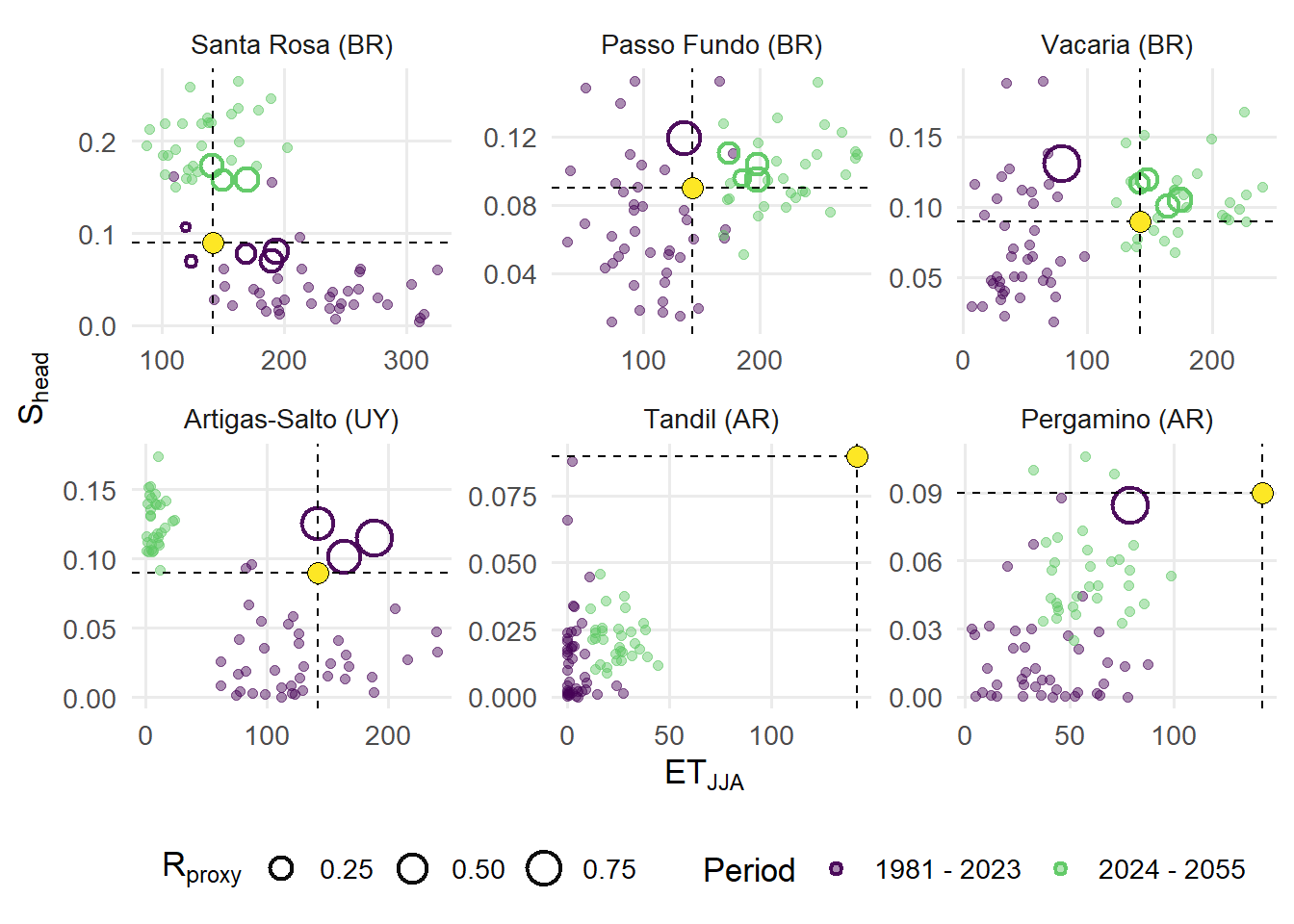
# Abs differences and Std vars -------------------------------------------------
df_all_subplot <- df_all %>%
  group_by(sentinel_id) %>%
  mutate(
    ET_JJA_2023 = ET_JJA[year == 2023][1],
    S_head_2023 = S_head[year == 2023][1],
    ET_JJA_Diff = ET_JJA - ET_JJA_2023,
    S_head_Diff  = S_head - S_head_2023,
    Flag = ET_JJA_Diff > 0 & S_head_Diff > 0,
    D_NE = ifelse(Flag, D, 0)
  ) %>%
  ungroup() %>%
  filter(year!=2023)

# Frequency Column bar
df_summary <- df_all_subplot %>%
  filter(!site %in% c("Tandil (AR)", "Pergamino (AR)")) %>%
  group_by(site, period) %>%
  summarise(freq = mean(analog_flag, na.rm = TRUE), .groups = "drop")
ColumPlot <- ggplot(df_summary, aes(x = period, y = freq, fill = period)) +
  geom_col(width = 0.5) +
  ylim(0,1) +
  geom_text(aes(label = round(freq, 2), color = period,),
            vjust = -0.5, size = 4.2, fontface = "bold") +
  scale_fill_viridis_d(end = 0.75) +
  scale_color_viridis_d(end = 0.75) +
  facet_wrap(~ site, nrow = 1) +
  labs(x = NULL, y = "Frequency") +
  theme_minimal() +
  theme(legend.position = "none")
ColumPlot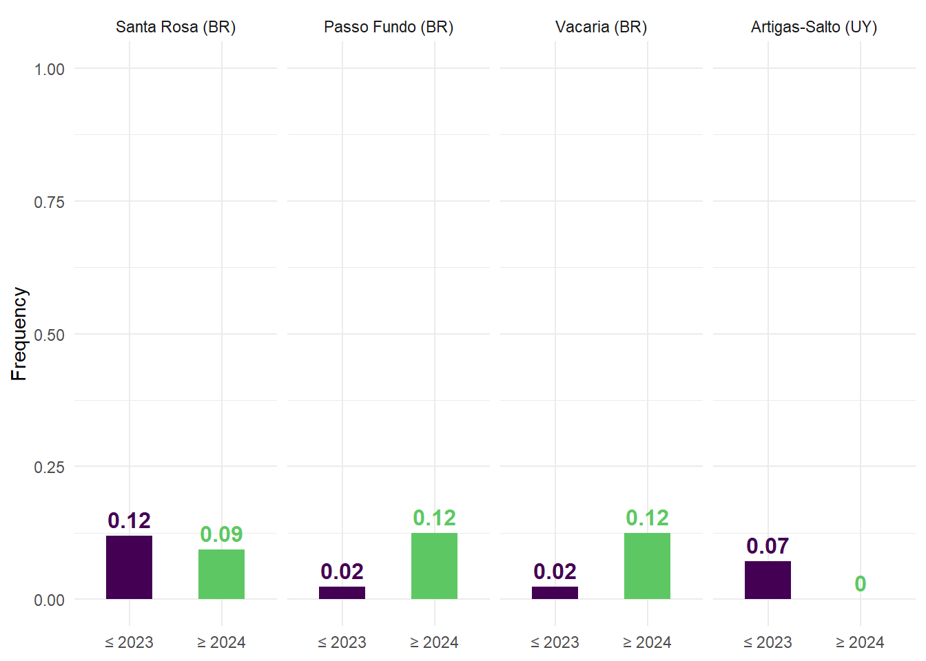
df_labels <- df_all_subplot %>%
  filter(!site %in% c("Tandil (AR)", "Pergamino (AR)")) %>%
  group_by(site, period) %>%
  summarise(
    freq = mean(D_NE > 0, na.rm = TRUE),
    .groups = "drop"
  ) %>%
  arrange(site, period) %>%
  group_by(site) %>%
  mutate(
    label = round(freq, 2),
    x_pos = ifelse(row_number() == 1, -Inf, Inf),   # left vs right
    hjust = ifelse(row_number() == 1, -0.1, 1.1)    # push inside
  ) %>%
  ungroup()

LinePlot <- ggplot(df_all_subplot %>%
                     filter(!site %in% c("Tandil (AR)", "Pergamino (AR)")),
  aes(x = year, y = D_NE, fill = period)) +
  geom_col(width = 1) +
  facet_wrap(~ site, nrow = 1) +
  scale_fill_viridis_d(end = 0.75) +
  scale_color_viridis_d(end = 0.75) +
  labs(
    x = "Year",
    y = bquote("Benchmark distance (" * D[PF~2023] * ")")
  ) +
  geom_text(
    data = df_labels,
    aes(
      x = x_pos,
      y = Inf,
      label = label,
      color = period,
      hjust = hjust
    ),
    inherit.aes = FALSE,
    vjust = 1.2,
    size = 4.2,
    fontface = "bold"
  )+
  theme_minimal() +
  theme(legend.position = "none")
LinePlot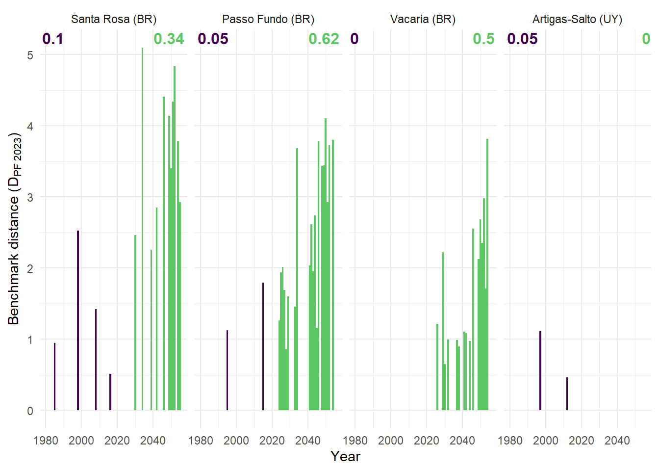
Plot <- p_pf_site / LinePlot / ColumPlot +
  plot_layout(heights = c(2, 1, 1)) +
  plot_annotation(tag_levels = "A") &
  theme(
    plot.tag = element_text(
      size = 16,
      face = "bold",
      color = "black"
    ),
    plot.tag.position = c(0.08, 0.99)
  )

ggsave( "RCP85_CrossSite.png",Plot,
       width = 8, height = 8, units = "in", dpi = 600)
Within site figure
df_era5 <- WithinSite_Era5_Indices %>%
  distinct() %>%
  mutate(
    analog_flag = analog_quantile & analog_distance,
    period = "≤ 2023"
  )

df_rcp85 <- WithinSite_RCP85_Indices %>%
  distinct() %>%
  mutate(
    analog_flag = analog_quantile & analog_distance,
    period = "≥ 2024"
  )
df_all <- bind_rows(df_era5, df_rcp85)
df_all <- df_all %>%
  mutate(site = factor(site, levels = c("Santa Rosa (BR)", "Passo Fundo (BR)", "Vacaria (BR)", "Artigas-Salto (UY)", "Tandil (AR)", "Pergamino (AR)")))

pf_benchmark <- df_era5 %>%
  dplyr::filter(year == CFG$benchmark_year)

pf_benchmark_era5_all <- df_era5 %>%
  filter(year == CFG$benchmark_year) %>%
  select(site, period, ET_JJA, S_head)%>%
  mutate(site = factor(all_sites, levels = levels(df_all$site)))
df_refs_all <- pf_benchmark_era5_all %>%
  select(site, period, ET_JJA, S_head)

p_pf_site <- ggplot() +

  # ===== Background points =====
  geom_point(
    data = df_all %>% filter(!analog_flag)%>% filter(year != 2023),
    aes(x = ET_JJA, y = S_head, color = period),
    alpha = 0.45,
    size  = 1.6
  ) +
  scale_color_viridis_d(end = 0.75, labels = c("≤ 2023" = "1981 - 2023", "≥ 2024" = "2024 - 2055")) +

  # ===== Analog points =====
  geom_point(
    data = df_all %>% filter(analog_flag) %>% filter(year!=2023),
    aes(x = ET_JJA, y = S_head, color = period, size = R_proxy),
    shape  = 21,
    stroke = 1.1,
    fill   = NA,
    alpha  = 0.95
  ) +

  # ===== Period-specific reference lines =====
  geom_vline(
    data = df_refs_all,
    aes(xintercept = ET_JJA),
    linetype = 2,
    show.legend = FALSE
  ) +

  geom_hline(
    data = df_refs_all,
    aes(yintercept = S_head),
    linetype = 2,
    show.legend = FALSE
  ) +

  # ===== Benchmarks =====
  geom_point(
    data = pf_benchmark_era5_all,
    aes(x = ET_JJA, y = S_head),
    shape = 21,
    size  = 4,
    stroke = 0.1,
    fill = viridis::viridis(100)[100]
  ) +

  # ===== Facet by site only =====
  facet_wrap(~ site, nrow = 2, scale="free") +

  labs(
    x = expression(ET[JJA]),
    y = expression(S[head]),
    color = "Period",
    size  = expression(R[proxy])
  ) +

  theme_minimal(base_size = 13) +
  theme(
    panel.grid.minor = element_blank(),
    legend.position = "right"
  )

p_pf_site <- p_pf_site +
  scale_x_continuous(n.breaks = 3) +
  theme(legend.position = "bottom")
p_pf_site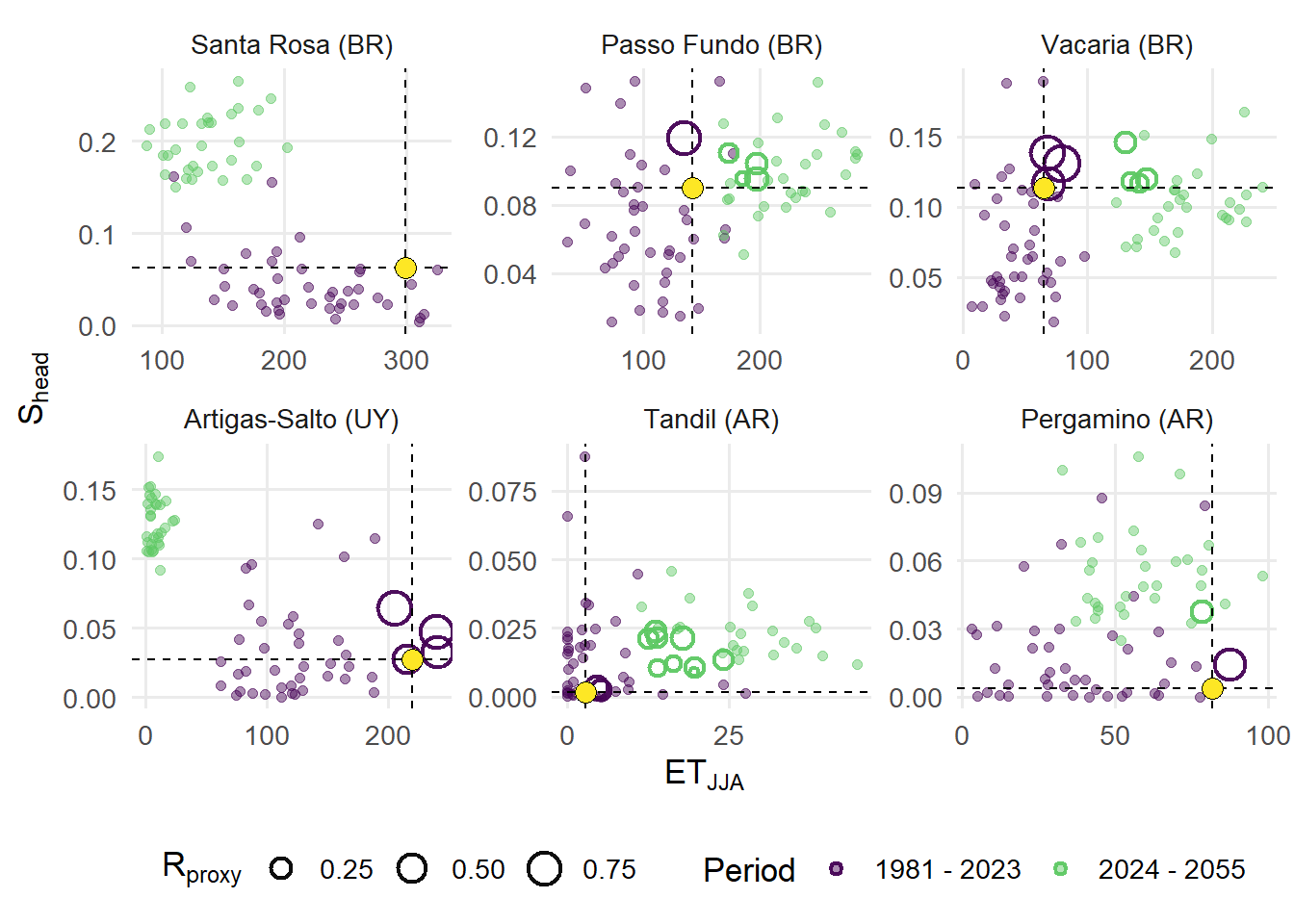
# Abs differences and Std vars -------------------------------------------------
df_all_subplot <- df_all %>%
  group_by(sentinel_id) %>%
  mutate(
    ET_JJA_2023 = ET_JJA[year == 2023][1],
    S_head_2023 = S_head[year == 2023][1],
    ET_JJA_Diff = ET_JJA - ET_JJA_2023,
    S_head_Diff  = S_head - S_head_2023,
    Flag = ET_JJA_Diff > 0 & S_head_Diff > 0,
    D_NE = ifelse(Flag, D, 0)
  ) %>%
  ungroup() %>%
  filter(year!=2023)

# Frequency Column bar
df_summary <- df_all_subplot %>%
  group_by(site, period) %>%
  summarise(freq = mean(analog_flag, na.rm = TRUE), .groups = "drop")
ColumPlot <- ggplot(df_summary %>% filter(!site %in% c("Santa Rosa (BR)")), aes(x = period, y = freq, fill = period)) +
  geom_col(width = 0.5) +
  geom_text(aes(label = round(freq, 2), color = period,), vjust = -0.5, size = 4.2, fontface = "bold") +
  scale_fill_viridis_d(end = 0.75) +
  scale_color_viridis_d(end = 0.75) +
  ylim(0,1)+
  facet_wrap(~ site, nrow = 1) +
  labs(x = NULL, y = "Frequency") +
  theme_minimal() +
  theme(legend.position = "none")
ColumPlot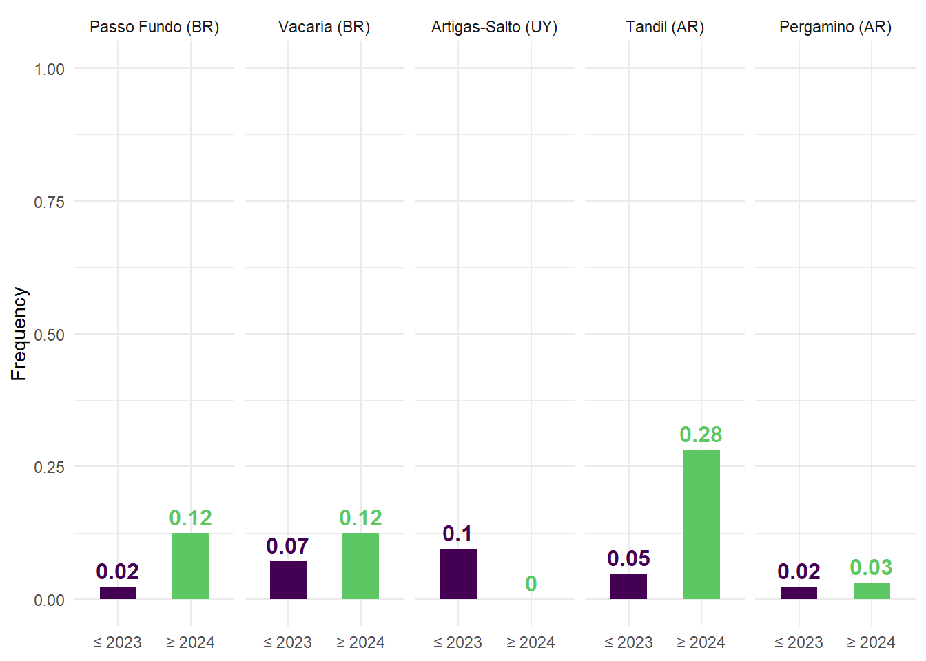
df_labels <- df_all_subplot %>%
  filter(!site %in% c("Santa Rosa (BR)")) %>%
  group_by(site, period) %>%
  summarise(
    freq = mean(D_NE > 0, na.rm = TRUE),
    .groups = "drop"
  ) %>%
  arrange(site, period) %>%
  group_by(site) %>%
  mutate(
    label = round(freq, 2),
    x_pos = ifelse(row_number() == 1, -Inf, Inf),   # left vs right
    hjust = ifelse(row_number() == 1, -0.1, 1.1)    # push inside
  ) %>%
  ungroup()

LinePlot <- ggplot(df_all_subplot %>% filter(!site %in% c("Santa Rosa (BR)")), aes(x = year, y = D_NE, fill = period)) +
  geom_col(width = 1) +
  ylim(0, 6)+
  facet_wrap(~ site, nrow = 1) +
  scale_fill_viridis_d(end = 0.75) +
  scale_color_viridis_d(end = 0.75) +
  labs(
    x = "Year",
    y = bquote("Benchmark distance (" * D[site~2023] * ")")
  ) +
  geom_text(
    data = df_labels,
    aes(
      x = x_pos,
      y = Inf,
      label = label,
      color = period,
      hjust = hjust
    ),
    inherit.aes = FALSE,
    vjust = 1.2,
    size = 4.2,
    fontface = "bold"
  )+
  theme_minimal() +
  theme(legend.position = "none")
LinePlot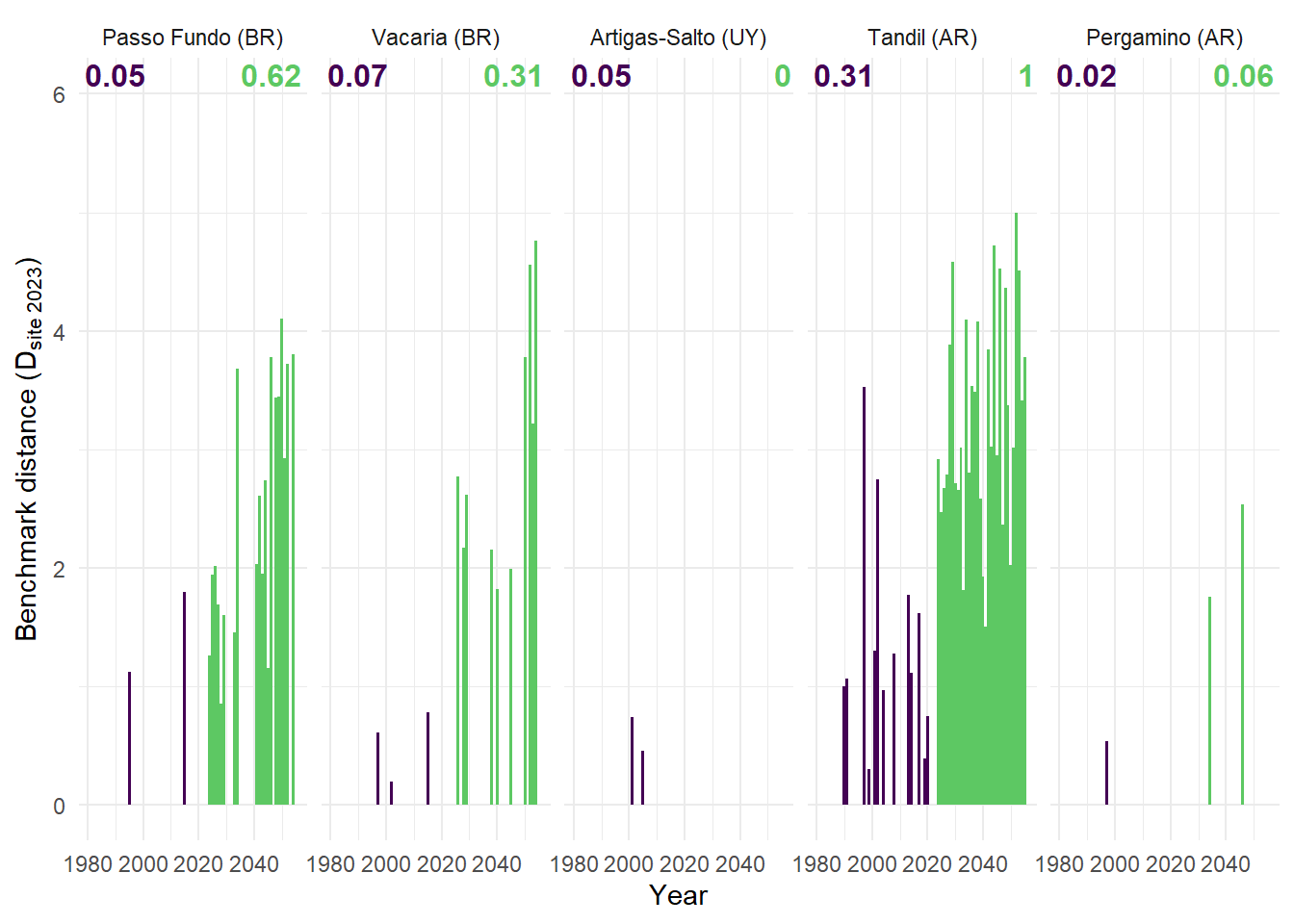
Plot <- p_pf_site / LinePlot / ColumPlot +
  plot_layout(heights = c(2, 1, 1)) +
  plot_annotation(tag_levels = "A") &
  theme(
    plot.tag = element_text(
      size = 16,
      face = "bold",
      color = "black"
    ),
    plot.tag.position = c(0.08, 0.99)
  )
ggsave( "RCP85_Whithin.png",Plot,
       width = 8, height = 8, units = "in", dpi = 600)
(A) Within-site bivariate distributions of yearly climate indices across six sentinel locations: Artigas-Salto (UY), Passo Fundo (BR), Pergamino (AR), Santa Rosa (BR), Tandil (AR), and Vacaria (BR). Points represent annual observations, colored by period. Colored rings represent years classified as analogs, with size corresponding to the Rproxy value. The x axis shows winter thermal exceedance (ETJJA), while the y axis shows heading-period thermo-hydric suitability (Shead).
(B) Euclidean distance to benchmark origin for the years both with climate indices greater than the benchmark, numbers indicate the relative frequency these years within each period.
(C) Relative frequency of analog years.
Suplemmentary Figs
Response functions to parameterize S_Head
# Parameters definition
pars <- list(RH0 = 90, k_RH = 2, T_low = 16, T_high = 26, k_T = 2)

# ---- data for curves ----
df_rh <- tibble(
  RH = seq(75, 100, by = 0.1),
  f  = f_RH(RH, RH0 = pars$RH0, k_RH = pars$k_RH)
)

df_t <- tibble(
  T  = seq(0, 40, by = 0.05),
  f  = f_T(T, T_low = pars$T_low, T_high = pars$T_high, k_T = pars$k_T)
)

# Panel A: humidity response
p_rh <- ggplot(df_rh, aes(RH, f)) +
  geom_line(linewidth = 0.9) +
  geom_vline(xintercept = pars$RH0, linetype = 2, linewidth = 0.5) +
  annotate("text", x = pars$RH0, y = 0.02,
           label = expression(RH[0] == 90*"%"),
           parse = TRUE, vjust = 0, hjust = -0.05, size = 3.2) +
  scale_y_continuous(limits = c(0, 1), breaks = seq(0, 1, 0.25)) +
  labs(
    x = "Mean relative humidity (RH, %)",
    y = expression(f[RH](RH))
  ) +
  theme_minimal(base_size = 11) +
  theme(panel.grid.minor = element_blank())

# Panel B: temperature response
p_t <- ggplot(df_t, aes(T, f)) +
  geom_line(linewidth = 0.9) +
  geom_vline(xintercept = c(pars$T_low, pars$T_high), linetype = 2, linewidth = 0.5) +
  annotate("text", x = (pars$T_low)-12, y = 0.9,
           label = expression(T[low] == 16*degree*C),
           parse = TRUE, vjust = 0, hjust = -0.05, size = 3.2) +
  annotate("text", x = (pars$T_high)+1, y = 0.9,
           label = expression(T[high] == 26*degree*C),
           parse = TRUE, vjust = 0, hjust = -0.05, size = 3.2) +
  scale_y_continuous(limits = c(0, 1), breaks = seq(0, 1, 0.25)) +
  labs(
    x = expression("Mean temperature ("*degree*C*")"),
    y = expression(f[T](T))
  ) +
  theme_minimal(base_size = 11) +
  theme(panel.grid.minor = element_blank())

# Figure layout
fig_S1 <- p_rh + p_t +

  plot_layout(guides = "collect")+
  plot_annotation(tag_levels = "A")

print(fig_S1)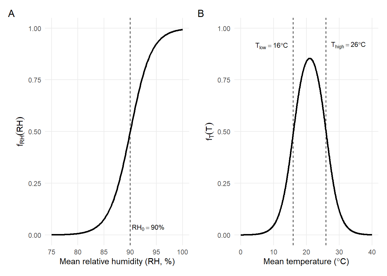
ggsave("S_HeadResponseCurves.png", fig_S1, width = 7.2, height = 3.2, dpi = 600, bg='white')(A) Logistic humidity response fRH(RH) centered at a high-humidity reference threshold (RH0=90%), representing progressively increasing suitability as relative humidity approaches saturation.
(B) Temperature response fT(T) defined as a bounded window between Tlow=16 ºC and Thigh=26 ºC, producing a bell-shaped curve with maximum suitability near the midpoint of the favorable thermal range. Both functions are scaled between 0 (unsuitable) and 1 (highly suitable).
Two-dimensional response surface of daily thermo-hydric suitability (Sd)
# Parameters definition
pars <- list(RH0 = 90, k_RH = 2, T_low = 16, T_high = 26, k_T = 2)

# Grid for surface
grid <- expand_grid(
  RH = seq(85, 100, by = 0.25),
  T  = seq(12, 30,  by = 0.1)
) %>%
  mutate(
    fRH = f_RH(RH, RH0 = pars$RH0, k_RH = pars$k_RH),
    fT  = f_T(T,  T_low = pars$T_low, T_high = pars$T_high, k_T = pars$k_T),
    S   = fRH * fT
  )

# Clean 2-D surface (heatmap)
p_surface <- ggplot(grid, aes(x = T, y = RH)) +
  geom_raster(aes(fill = S), interpolate = TRUE) +
  geom_contour(aes(z = S), color = "grey25", linewidth = 0.25, bins = 6) +
  geom_hline(yintercept = pars$RH0, linetype = 2, linewidth = 0.4) +
  geom_vline(xintercept = c(pars$T_low, pars$T_high), linetype = 2, linewidth = 0.4) +
  scale_fill_viridis_c(limits = c(0, 1), direction = -1, option = "D") +
  labs(
    x = expression("Mean temperature ("*degree*C*")"),
    y = "Mean relative humidity (RH, %)",
    fill = expression(S[d])
  ) +
  theme_minimal(base_size = 12) +
  theme(
    panel.grid.minor = element_blank(),
    legend.position = "right"
  )
print(p_surface)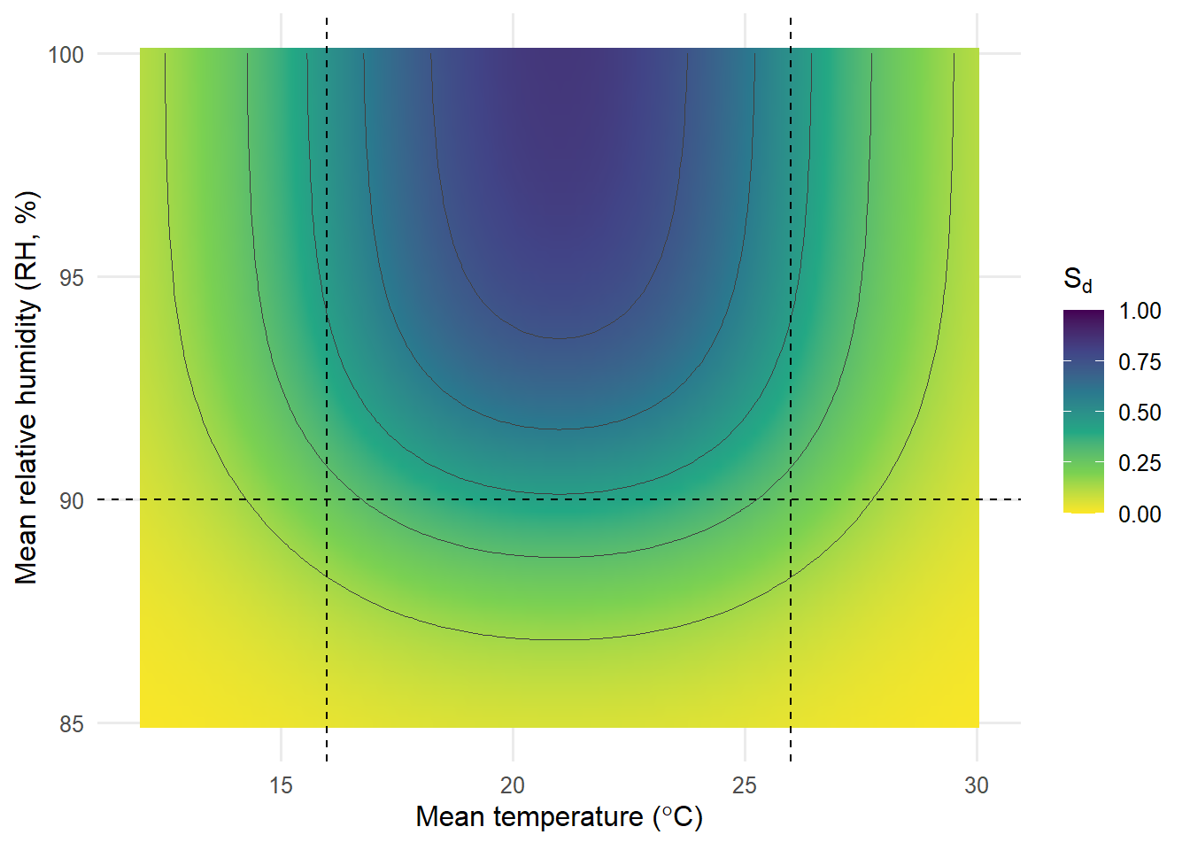
ggsave("SdResponseSurface.png", p_surface, dpi = 600, bg='white')